Making my ODE solver solve ODEs

◀

Soil:

Making a Pyhton Library to Solve Differential Equations

By: Alfie Chadwick Date: January 12, 2024 flower

▶

Seeds:

After writing out the last post where I wrote out a python library for using an improved version of Euler’s method to solve ODEs. But so far, we haven’t been solving ODES, instead we have just been taking an initial value and iterating it over the length of a domain. To To make the ODE estimator work, we need to ensure that the conditions of the ODE are met at each step.

Simplifying ODEs: Constant-Linear ODEs

ODEs are often categorized as linear or non-linear. Linear ODEs take the form $a_0(x)y+a_1(x)y^{\prime }+...+a_n(x)y^n=b(x)$, with both $a$ and $b$ representing functions of $x$, while Non-linear equations are all the others. In our solver’s context, we’ll concentrate on a subset I’ve termed “constant-linear” ODEs, characterized by constant coefficients for $y$ terms and a linear function of $x$ for $b$. Specifically, a constant-linear ODE looks like $a_{0}y+a_1{y}^{\prime }+...+a_n{y}^n=bx+c$.

This may seem like a very restrictive requirement, but there are many famous examples of this kind of equation including:

1. Simple Harmonic Motion: $$y^{″}+{\omega }^{2}y=0$$

2. Radioactive Decay: $$\frac{dy}{dt}=-\lambda y$$

3. RC Circuit Equation: $$y^{\prime }+\frac{1}{RC}y=0$$

4. Damped Harmonic Oscillator: $$y^{″}+2\gamma y^{\prime }+{\omega }_0^{2}y=0$$

5. Heat Equation (One-Dimensional): $$u^{″}-\frac{1}{\alpha }{u}^{\prime }=0$$

6. Exponential Growth or Decay: $$y^{\prime }=ky$$

A Quick Diversion: ODEs in Vector Space

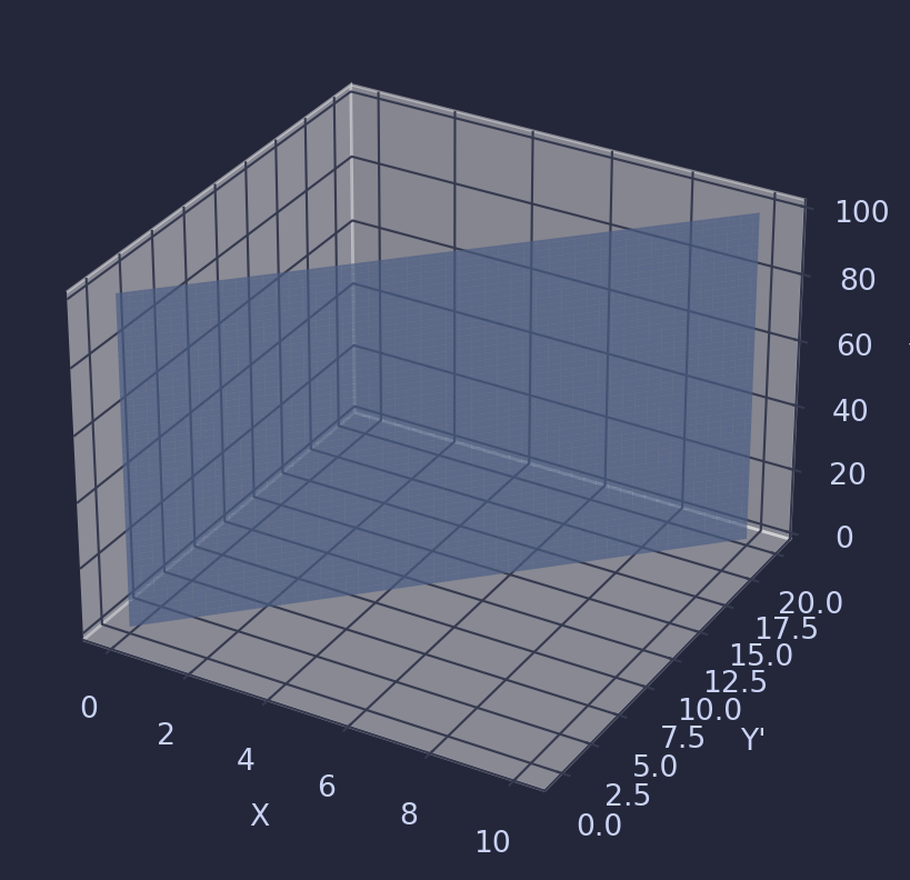
Pivoting for a moment, I want to take a quick moment to reframe how we are imagining ODEs. Most of the time, we see ODEs as curves in space and/or time, but I want to reframe them as planes in a vector space.

Each point in this vector space describes the state of a point along a curve, such that a values of the vector give:

$$\left[\begin{array}{c}1\\ x\\ y(x)\\ y^{\prime }(x)\\ y^{″}(x)\\ ...\\ y^n(x)\end{array}\right]$$

This means that an ODE can be defined by a plane that contains all the points which meet the requirements of the ODE.

For example, for the equation $y^{\prime }=2x$ this plane looks like:

import matplotlib.pyplot as plt
import numpy as np
import matplotlib as mpl
import matplotlib.pyplot as plt
from mpl_toolkits.mplot3d import Axes3D
import catppuccin
mpl.style.use(catppuccin.PALETTE.macchiato.identifier)

# Create a grid of values for x and y
x = np.linspace(0, 10, 100)
y = np.linspace(0, 100, 100)
x, y = np.meshgrid(x, y)

# Calculate corresponding z
z = (2*x)

# Create a figure and a 3D axis
fig = plt.figure()
ax = fig.add_subplot(111, projection='3d')
ax.plot_surface(x, z,y, alpha = 0.7)

# Set labels
ax.set_xlabel('X')
ax.set_zlabel('Y')
ax.set_ylabel("Y'")

# Show the plot
plt.show()

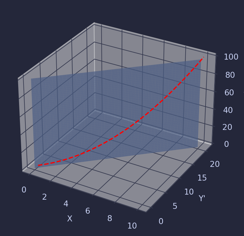
Then a specific solution to the ODE exists as a curve that sits on this plane. For example, for the IVP that starts at (0,0), the solution follows this curve:

Lx = np.linspace(0, 10, 100)
Ly = np.array([x**2 for x in Lx])

# Create masks for the conditions
mask = (Lx <= 10) & (Lx >= 0) & (Ly <= 100) & (Ly >= 0)

# Now apply the mask to both arrays to exclude unwanted values
filtered_Lx = Lx[mask]
filtered_Ly = Ly[mask]

Lz = (2*filtered_Lx) +1

# Create a new figure
fig = plt.figure()
ax = fig.add_subplot(111, projection='3d',computed_zorder=False)

# Plot surface and line
ax.plot_surface(x, z,y, zorder=0,alpha = 0.7)
ax.plot(filtered_Lx, Lz, filtered_Ly, color='r',linestyle='dashed' , zorder=1)


# Set labels
ax.set_xlabel('X')
ax.set_zlabel('Y')
ax.set_ylabel("Y'")

# Show the plot
plt.show()

But Why Does This Matter

The reason that we want to reframe ODEs in this way is because of the following fact:

For all constant-linear ODEs, we can express the ODE as a matrix such that applying it to any point in the vector space would map any point to a valid point on the curve defined by the ODE

Looking at the equations above, these matrices ($T$) are:

1. Simple Harmonic Motion: $$T=\left[\begin{array}{ccccc}1& 0& 0& 0& 0\\ 0& 1& 0& 0& 0\\ 0& 0& 1& 0& 0\\ 0& 0& 0& 1& 0\\ 0& 0& -{\omega }^2& 0& 0\end{array}\right]$$

2. Radioactive Decay: $$T=\left[\begin{array}{cccc}1& 0& 0& 0\\ 0& 1& 0& 0\\ 0& 0& 1& 0\\ 0& 0& -\lambda & 0\end{array}\right]$$

3. RC Circuit Equation: $$T=\left[\begin{array}{cccc}1& 0& 0& 0\\ 0& 1& 0& 0\\ 0& 0& 1& 0\\ 0& 0& \frac{-1}{RC}& 0\end{array}\right]$$

4. Damped Harmonic Oscillator: $$T=\left[\begin{array}{ccccc}1& 0& 0& 0& 0\\ 0& 1& 0& 0& 0\\ 0& 0& 1& 0& 0\\ 0& 0& 0& 1& 0\\ 0& 0& -{\omega }^2& -2\gamma & 0\end{array}\right]$$

5. Heat Equation (One-Dimensional): $$T=\left[\begin{array}{ccccc}1& 0& 0& 0& 0\\ 0& 1& 0& 0& 0\\ 0& 0& 1& 0& 0\\ 0& 0& 0& 1& 0\\ 0& 0& 0& \frac{1}{\alpha }& 0\end{array}\right]$$

6. Exponential Growth or Decay: $$T=\left[\begin{array}{cccc}1& 0& 0& 0\\ 0& 1& 0& 0\\ 0& 0& 1& 0\\ 0& 0& k& 0\end{array}\right]$$

Using these to fit ODEs

Now that we can express the ODEs in the form of a matrix, we can implement these matriexies in the ODE solver package to make the solution fit the ode. It’s important here to note that I’ve diverted from my old definitions of $Y$ here, where the first element of the vector is $y(x)$.

To make a step in the approximation we use the following equation:

$$\left[\begin{array}{c}1\\ x+h\\ y(x+h)\\ y^{\prime }(x+h)\\ y^{″}(x+h)\\ ...\\ y^n(x+h)\end{array}\right]=S\cdot \left[\begin{array}{c}1\\ x\\ y(x)\\ y^{\prime }(x)\\ y^{″}(x)\\ ...\\ y^n(x)\end{array}\right]ϵ$$

Where $S$ is: $$\left[\begin{array}{ccccccc}1& 0& 0& 0& 0& ...& 0\\ h& 1& 0& 0& 0& ...& 0\\ 0& 0& 1& \frac{h}{1!}& \frac{h^2}{2!}& ...& \frac{h^n}{n!}\\ 0& 0& 0& 1& \frac{h}{1!}& ...& \frac{h^{n-1}}{(n-1)!}\\ 0& 0& 0& 0& 1& ...& \frac{h^{n-2}}{(n-2)!}\\ ...& ...& ...& ...& ...& ...\\ 0& 0& 0& 0& 0& ...& 1\end{array}\right]$$

When making this step, the error in the approximation will move the point away from the plane that contains all valid solutions to the ODE, and therefore we will have to snap it back using one of the transformation matrices ($T$).

Implementing this method in our python library:

def expanded_euler(dims, h):
    step_matrix = np.zeros((dims, dims))
    for i in range(dims):
        for j in range(i, dims):
            # Is 1, and h at j-i =0, 1 respectively
            step_matrix[i, j] = h ** (j - i) / math.factorial(j - i)
    expanded_matrix = add_x_and_1(step_matrix, h)
    return expanded_matrix


def add_x_and_1(original_matrix, h):
    new_size = len(original_matrix) + 2
    new_matrix = np.zeros((new_size, new_size), dtype=original_matrix.dtype)

    # Set the 2x2 top left matrix
    new_matrix[0:2, 0:2] = [[1, 0], [h, 1]]

    # Copy the original matrix to the bottom right of the new matrix.
    new_matrix[2:, 2:] = original_matrix
    return new_matrix


def linear(y, step_matrix_generator, transformation_matrix, steps=10, h=0.1):
    dims = len(y) - 2
    step_matrix = transformation_matrix @ step_matrix_generator(dims, h)
    output_list = []

    y_n = y.copy()
    i = 0
    while i < steps:
        y_n = step_matrix @ y_n
        output_list.append(y_n)
        i += 1

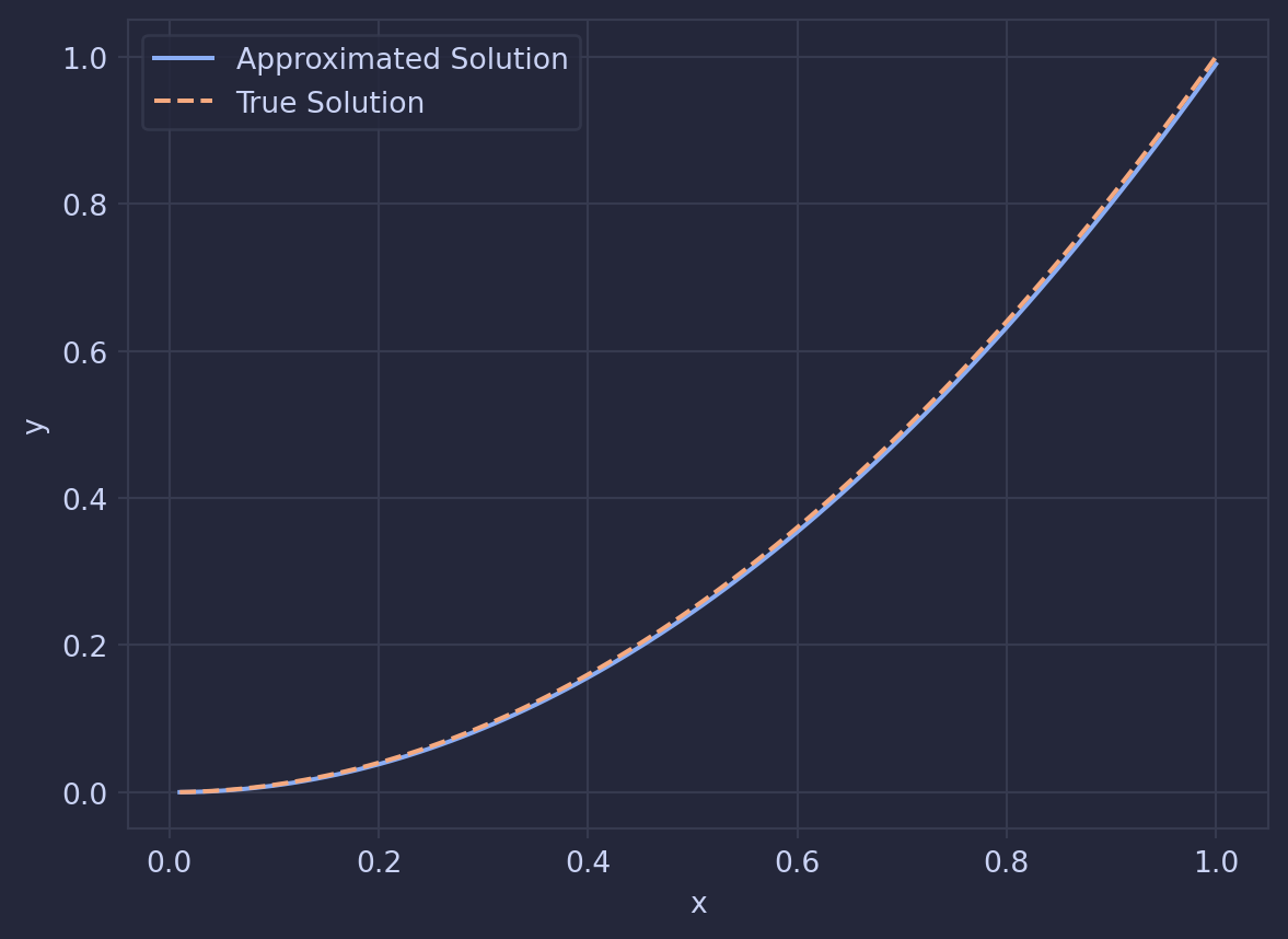
Bind this machinery together, and you get a tool capable of tackling the initial example of $y^{\prime }=2x$ passing through the point (0,0):

import numpy as np
import math


class Solution:
    def __init__(self, input_list: list):
        solution_list = sorted(input_list, key=lambda x: x[1])

        dims = len(solution_list[0]) - 2
        self.x = np.array([x[1] for x in input_list])

        value_lists = [[] for _ in range(dims)]

        for v in input_list:
            for i in range(dims):
                value_lists[i].append(v[i + 2])

        for i in range(dims):
            self.__dict__[f"y_{i}"] = np.array(value_lists[i])

    def interpolate(self, x, y_n):
        """
        allows you to get any value from the solution by interpolating the points

        """
        y_values = self.__dict__[f"y_{y_n}"]

        x_max_index = np.where(self.x >= x)[0][0]
        x_min_index = np.where(self.x <= x)[0][-1]

        x_at_x_max = self.x[x_max_index]
        x_at_x_min = self.x[x_min_index]

        y_at_x_max = y_values[x_max_index]
        y_at_x_min = y_values[x_min_index]

        slope = (y_at_x_max - y_at_x_min) / (x_at_x_max - x_at_x_min)

        value = y_at_x_min + slope * (x - x_at_x_min)
        return value

def linear(y, step_matrix_generator, transformation_matrix, steps=10, h=0.1):
    dims = len(y) - 2
    step_matrix = transformation_matrix @ step_matrix_generator(dims, h)
    output_list = []

    y_n = y.copy()
    i = 0
    while i < steps:
        y_n = step_matrix @ y_n
        output_list.append(y_n)
        i += 1

    return Solution(output_list)

init_y = [1,0,0,0] #[1,x,y,y']
transformation_matrix = np.array([
   [ 1,0,0,0 ],
   [ 0,1,0,0 ],
   [ 0,0,1,0 ],
   [ 0,2,0,0 ]
])
solution = linear(
    init_y,
    expanded_euler,
    transformation_matrix,
    steps=100, h=0.01)

plt.plot(solution.x, solution.y_0, label='Approximated Solution')
plt.plot(solution.x, solution.x**2, label='True Solution', linestyle='--')
plt.xlabel('x') # Label for the x-axis
plt.ylabel('y') # Label for the y-axis
plt.grid(True) # Show a grid for better readability
plt.legend()
plt.show()

What’s Next?

This method seems to work pretty well and follows the true solution pretty closely. I’m going to stop here for now but there are many things on my wishlist that I want to build in later posts. This includes:

• Solving IVPs which aren’t constant-linear
• Solving BVPs
• Applying this method to PDEs

Stay tuned for more posts in this series where I try to implement these features into my solver!