import numpy as np
import math


def euler(dims, h):
    # Start with an identity matrix
    step_matrix = np.identity(dims)
    # Add in all the h values
    for i in range(dims - 1):
        step_matrix[i, i + 1] = h
    return step_matrix


def expanded_euler(dims, h):
    step_matrix = np.zeros((dims, dims))
    for i in range(dims):
        for j in range(i, dims):
            # Is 1, and h at j-i =0, 1 respectively
            step_matrix[i, j] = h ** (j - i) / math.factorial(j - i)
    return step_matrix
Making a Python Library to solve differential Equations
◀
By: Alfie Chadwick
Date: December 29, 2023
Flower
▶
After having the initial idea I wrote up in a previous post, I thought it was a good idea to turn it into a python library so that I can use it as part of my other projects.
It also gives me a chance to see numerically how well the new method works compared to the Euler method.
First Steps
So in the last post I set out the method such that:
\[ \begin{bmatrix} y(x+h)\\ y'(x+h)\\ y''(x+h)\\ ...\\ y^{n}(x+h)\\ \end{bmatrix} = S \cdot \begin{bmatrix} y(x)\\ y'(x)\\ y''(x)\\ ...\\ y^{n}(x)\\ \end{bmatrix} + \epsilon \]
In the Euler method, \(S\) is:
\[ \begin{bmatrix} 1 & h & 0 & ... & 0\\ 0 & 1 & h & ... & 0\\ 0 & 0 & 1 & ... & 0\\ ... & ... & ... & ... & ...\\ 0 & 0 & 0 & ... & 1\\ \end{bmatrix} \]
And in the new method I proposed, \(S\) is now:
\[ \begin{bmatrix} 1 & \frac{h}{1!} & \frac{h^2}{2!} & ... & \frac{h^n}{n!}\\ 0 & 1 & \frac{h}{1!} & ... & \frac{h^{n-1}}{(n-1)!}\\ 0 & 0 & 1 & ... & \frac{h^{n-2}}{(n-2)!}\\ ... & ... & ... & ... & ...\\ 0 & 0 & 0 & ... & 1\\ \end{bmatrix} \]
Converting these matrices into python is fairly easy.
Making a step simulation
Now that we have the stepping matrices, we can use them to iterate from an initial value. All we have to do is generate the stepping matrix for the given problem, and then for each step, we just multiple the previous step by the stepping matrix.
def IVP(x, y, step_matrix_generator, steps=10, h=0.1):
    dims = len(y)
    step_matrix = step_matrix_generator(dims, h)
    output_dict = {x: y}

    x_n = x
    y_n = y.copy()
    i = 0
    while i < steps:
        y_n = step_matrix @ y_n
        x_n += h
        output_dict[x_n] = y_n
        i += 1

    return output_dict
Testing and Comparing the methods
Now we can run the simulations, let’s see how good they are. Say you throw a ball up in the air and track its vertical position. The path of the ball is described by the equation \(y'' = -9.8\). We can know for a fact that the solution to this equation is \(\frac{-9.8}{2}x^2+V_0x+P_0\), where \(V_0\) is the initial velocity and \(P_0\) is the initial position. So now lets compare the real solutions to the simulations.
# Time starts at 0
x = 0
# Start the object moving upwards with a velocity of 10
y = np.array([0, 10, -9.8])

euler_result = IVP(x, y, euler)
expanded_euler_result =IVP(x, y, expanded_euler)
true_result = {x: np.array([
                    -4.9 * x**2 + 10 * x,
                    -9.8 * x + 10,
                    -9.8
                ]) for x in np.arange(0, 1.1, 0.1)}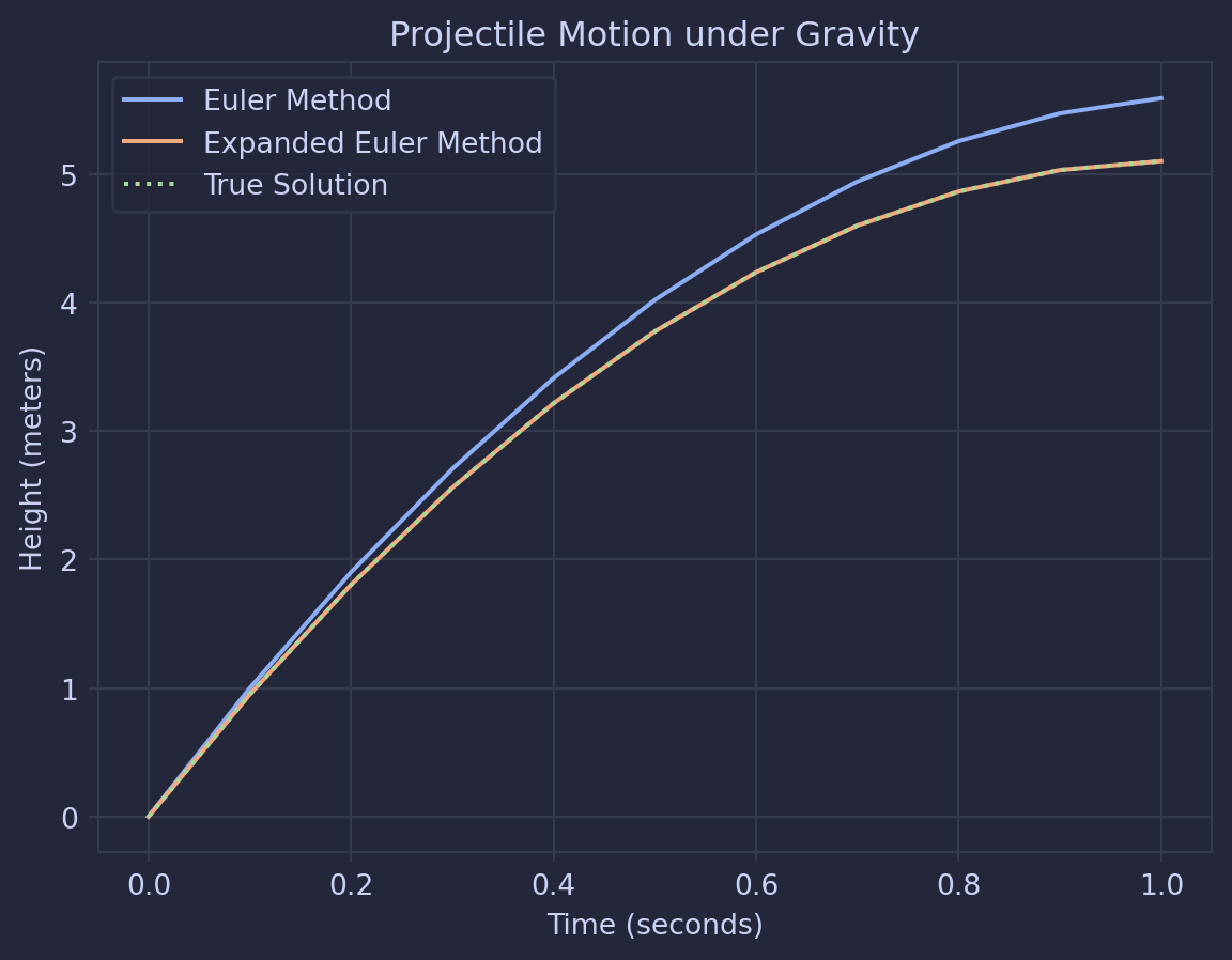
So from here, we’re looking pretty good. The new method is much closer to the true solution than the Euler method in in this scenario. However, when working with numerical methods, it generally isn’t too hard to improve the accuracy of the model, but there will be a trade off in computation time. So lets see how much longer it takes to compute the approximation with the expanded method comparing it to the original.
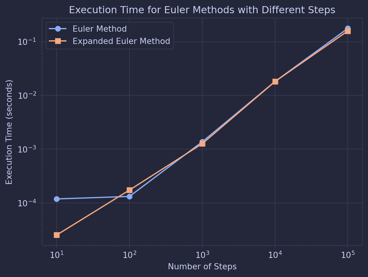
Looking at this graph, we can see that we’re not sacrificing compute time for better accuracy, so this seems like a big win, though I haven’t optimised the Euler method that much. But overall, the new method seems to show some promise in approximating differential equations.